DRAFT - The Extended One-Layer Model

The ABCs of the greenhouse effect… thermal and not fluorescence

In the single-layer model, the greenhouse effect is explained by the interaction of two plates that behave like black bodies. This model is taught at various universities and disseminated by academic institutions. It is considered the ABC of the greenhouse effect. See for example (Dufresne and Treiner 2011).

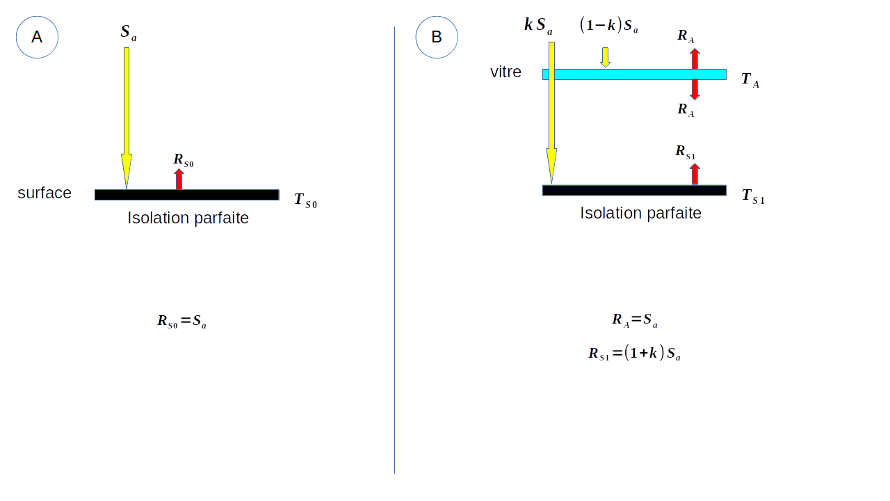
This model produces excessively high surface temperature values. A parameter k describing the degree of transparency of the atmosphere is introduced. It allows this model to be adjusted to observations. See Figure 1.

Given

$S$	The solar radiation at the top of the atmosphere	1368 W m-2
$A$	The albedo of the planet	0.3
$S_a=(1-A)S/4$	The average solar radiation absorbed by the Earth’s surface	239 W m-2
${ϵ}_S$	The emissivity of the Earth’s surface
${ϵ}_A$	The emissivity of the atmosphere
$\sigma$	The Stefan-Boltzmann constant (SB)	5.67 10-8 W m-2 °K-4
$T_{S0}$	The temperature of the Earth’s surface in the absence of an atmosphere	255 °K
$T_{S1}$	The temperature of the Earth’s surface in the presence of an atmosphere	292 °K
$T_A$	The average temperature of an atmosphere concentrated in a single layer	K
$R_{S0}$	The radiation emitted by the Earth’s surface in the absence of an atmosphere
$R_{S1}$	Radiation emitted by the Earth’s surface in the presence of an atmosphere
$R_A$	The radiation emitted by the atmosphere upwards and downwards
$k$	The degree of transparency of the atmosphere	$0<=k<=1$

Note: The value $T_{S1}=292°K$ is the current value of the average ocean surface temperature (NOAA OI V2 time series)

Figure 1: Panel A corresponds to an Earth without an atmosphere. The Earth’s surface is likened to a black/grey body whose underside is perfectly insulated (black rectangle). In panel B, the atmosphere is likened to a window (blue rectangle). This window is a black/grey body that is partially transparent to solar radiation, but opaque to IR radiation emitted by the Earth’s surface.

For a black body Earth without atmosphere, the thermal balance is written (received flux = emitted flux):

$$\begin{array}{}\text{(1)}& S_a=R_{S0}={ϵ}_S\sigma T_{S0}^4\end{array}$$

We deduce from this

$$\begin{array}{}\text{(2)}& T_{S0}=\sqrt[4]{\frac{S_a}{{ϵ}_S\sigma }}\end{array}$$

For an Earth with an atmosphere, we must write the thermal balance of each plate.

For the Earth’s surface, we have:

$$\begin{array}{}\text{(3)}& k{S}_a+R_A=R_{S1}\end{array}$$

In a similar way, we have for the atmosphere:

$$\begin{array}{}\text{(4)}& \begin{array}{rl}(1-k)S_a+R_{S1}& =2R_A\\ \frac{1}{2}[(1-k)S_a+R_{S1}]& =R_A\end{array}\end{array}$$

By injecting Equation 4 into Equation 3, it comes

$$\begin{array}{}\text{(5)}& k{S}_a+\frac{1}{2}[(1-k)S_a+\sigma T_{S1}^4]=\sigma T_{S1}^4\end{array}$$

And so

$$\begin{array}{}\text{(6)}& R_{S1}=(1+k)S_a\end{array}$$

By injecting this value into Equation 3, we obtain

$$\begin{array}{}\text{(7)}& R_A=S_a\end{array}$$

$R_A$ and $R_{S1}$ do not depend on the emissivities, and $R_A$ does not depend on the degree of transparency $k$.

The temperatures are obtained by applying SB’s law.

For the surface:

$$\begin{array}{}\text{(8)}& \begin{array}{rl}{T}_{S1}& =\sqrt[4]{1+k}\sqrt[4]{\frac{S_a}{{ϵ}_S\sigma }}\\ & =\sqrt[4]{1+k}{T}_{S0}\end{array}\end{array}$$

The value of $T_{S1}$ is largest when $k=1$.

For the atmosphere:

$$\begin{array}{}\text{(9)}& T_A=\sqrt[4]{\frac{S_a}{{ϵ}_A\sigma }}\end{array}$$

Pour une atmosphère complètement transparente, $k=1$ et une émissivité ${ϵ}_S$ de 1, et on retrouve la valeur publiée dans Dufresne and Treiner (2011):

$$T_{S1}=\sqrt[4]{2}{T}_{S0}=303°K$$

This value is significantly higher than observed.

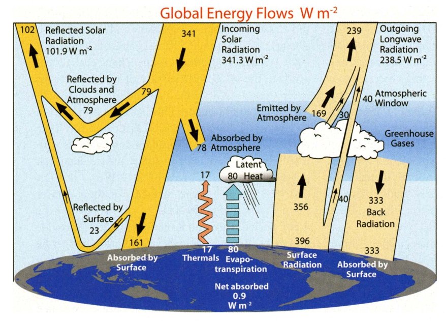
With the observed average temperature of 292°C and a commonly accepted value of ${ϵ}_S=0.97$, the radiation emitted by the surface $R_{S1}=400W/M^2$. Using Equation 6, we deduce $k=400/239-1=0.673$. The portion of solar radiation absorbed by the atmosphere is $(1-0.673)\ast 239=78W/M^2$. These exact figures are found in the Trenberth diagram, which was derived using a more complicated and completely different approach! See Figure 2 extracted from Trenberth, Fasullo, and Kiehl (2009).

Figure 2: Trenberth diagram

In this model, back-radiation is equal to the average absorbed solar radiation, i.e., 239 W/M² , regardless of the value of $k$. It is thermal in nature. It is black/gray body radiation following the SB law caused by electric dipole oscillations within matter. This radiation has nothing to do with the fluorescence radiation characteristic of greenhouse gases (GHGs).

In the atmosphere, only liquid or solid water present in clouds is capable of emitting SB-type thermal radiation. GHG molecules other than water exist only in gaseous form in the atmosphere. Gaseous molecules do not emit thermal radiation.

The interpretation of the Trenberth diagram in light of this thermal model can be found here.

In Dufresne and Treiner (2011), the effect of an increase in GHGs is simulated by increasing the number of plates. In a model with n isothermal plates, the temperature of the top one is unchanged, and that of the bottom increases indefinitely with the number of plates. The same is true for the temperature gradient between the first and last plates, which has nothing to do with the adiabatic gradient observed in the troposphere. This model with N plates is completely unrealistic.

In the Figure 1, if air containing GHGs were introduced between the two plates, each plate would be subject to back-radiation and would therefore have to heat up. In this case, the energy balance would no longer be balanced. It is impossible for GHGs, which have no warming power, to create such an imbalance. The energy balance of each plate cannot change. For each plate, the back-radiation will either be absorbed and re-emitted, or reflected, but without any change in temperature.

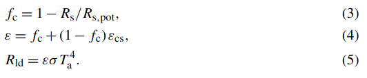
The essentially thermal nature of back-radiation is described in sections 5.4.1 and 5.4.2 in Monteith and Unsworth (2013). The formula 5.30 proposed there to estimate back-radiation is very explicit:

In a comprehensive study of back-radiation (Tian et al. (2023)) based on FLUXNET observations, the NASA-CERES dataset, and the ERA5 reanalysis, the authors conclude that heat accumulated in the lower atmosphere is the main source of diurnal and seasonal variations in back-radiation. Formulas 3, 4, and 5, which they use in their analyses and which produce excellent correlations, leave no doubt: the lower atmosphere behaves like a gray body.

References

Dufresne, Jean-Louis, and Jacques Treiner. 2011. “L’effet de Serre Atmosphérique: Plus Subtil Qu’on Ne Le Croit!” Le Bup 105 (936): 821–40. https://www.hprevot.fr/plus-subtil.pdf.

Monteith, John, and Mike Unsworth. 2013. Principles of Environmental Physics: Plants, Animals, and the Atmosphere. Academic press. https://dlib.scu.ac.ir/bitstream/Hannan/388077/2/9780123869104.pdf.

Tian, Yinglin, Deyu Zhong, Sarosh Alam Ghausi, Guangqian Wang, and Axel Kleidon. 2023. “Understanding Variations in Downwelling Longwave Radiation Using Brutsaert’s Equation.” Earth System Dynamics 14 (6): 1363–74. https://esd.copernicus.org/articles/14/1363/2023/esd-14-1363-2023.pdf.

Trenberth, Kevin E, John T Fasullo, and Jeffrey Kiehl. 2009. “Earth’s Global Energy Budget.” Bulletin of the American Meteorological Society 90 (3): 311–24. https://journals.ametsoc.org/view/journals/bams/90/3/2008bams2634_1.xml.