DRAFT - Transfer by successive bounces
Bypassing the absorption bands by successive rebounds.
1 Principes
L’approche décrite dans ce document permet de comprendre comment la surface terrestre peut évacuer toute l’énergie solaire qu’elle a absorbée en présence d’une atmosphère contenant des GES.
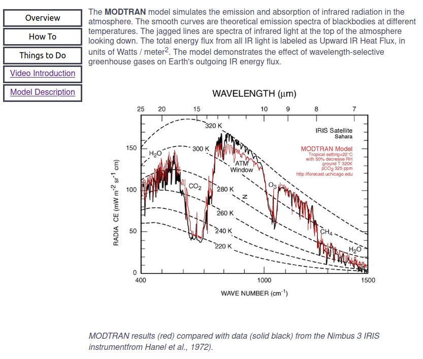
Si une fraction k d’une émission de la surface de la Planète est systématiquement renvoyée par l’atmosphère, elle sera réémise par la surface qui fera l’objet d’un nouveau renvoi partiel. Comme la réémission se fait dans toute la gamme des longueurs d’onde, les bandes d’absorption des GES sont contournées par des rebonds successifs qui ne nécessitent aucun changement de température. Le calcul est détaillé dans la Table 1 et la Fig. 1.
| Iteration | Emission | Return | Net emission |
|---|---|---|---|
| 1 | 1 | k | 1-k |
| 2 | k | k2 | k(1-k) |
| 3 | k2 | k3 | k2(1-k) |
| 4 | k3 | k4 | k3(1-k) |
| … | … | … | … |
The sum of net emissions is equal to (1-k)(1+k+k2+k3+…).
The infinite sum of the second factor is equal to the series expansion of 1/(1-k), and the sum of the net emissions is therefore equal to (1-k) * 1/(1-k) = 1.
The total back-radiation is equal to the sum of the returns. It is worth k * (1+k+k2+k3+…) = k/(1-k).
The sum of the emissions is equal to 1+k+k2+k3+… = 1/(1-k)
Therefore, GHGs do not create any heat accumulation in the Earth-Atmosphere system. The absorbed energy is evacuated following a tortuous path, but ultimately, all the absorbed energy is returned to the Cosmos. The radiative forcing of GHGs imagined by the IPCC is zero.
2 Concrete example
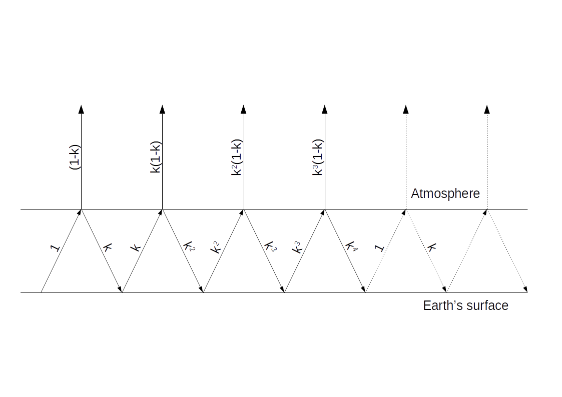
Let’s take a concrete example based on the online simulator MODTRAN from the University of Chicago which allows us to calculate the distribution of infrared radiation in the atmosphere. See Fig. 2.
The 1976 U.S. Standard Atmosphere was selected; all other options were left at their default values.
The jagged blue curve is intended to represent the IR radiation escaping from the atmosphere observed by an observer located at an altitude of 70 km. However, it only represents the first back and forth between the Earth’s surface and the atmosphere.
The smooth curves of different colors correspond to graybody radiation intensities at different temperatures.
The button Show Raw Model Output allows to retrieve the parameters and the results of the calculation. These were completed by the recursive calculation by multiple bounces. See Fig. 3.
The ratio of the area under the blue curve to that under the red curve is 0.705, which gives a value of f = 1 - 0.705 = 0.295. It is not necessary to perform a calculation by successive iterations to determine the green curve. To obtain it, simply multiply the blue curve by 1/(1 - f) = 1/0.705 = 1.418.
The areas under the green and red curves are then identical. This must be the case, otherwise the planet’s energy balance is not balanced.
The blue curve is supposed to correspond to the measurements of an observer located at an altitude of 70 km. How can anyone believe for a single instant that this could be true? The model chosen corresponds to current conditions on Earth with an average surface temperature of 15 °C (288.2 °K) and current GHG concentrations (400 ppm for CO2 ). The Earth has had plenty of time to adapt its temperature to solar radiation and GHGs. It is impossible that we are observing a radiation deficit of 29.5% today. The Earth is currently almost in thermal equilibrium. According to the IPCC, at the top of the atmosphere, absorbed solar radiation is 240 W/M2 and outgoing IR radiation is 239.1 W/M2. See figures 7.2 and 7.3 in the Chapter 7 of IPCC AR6 WG1.
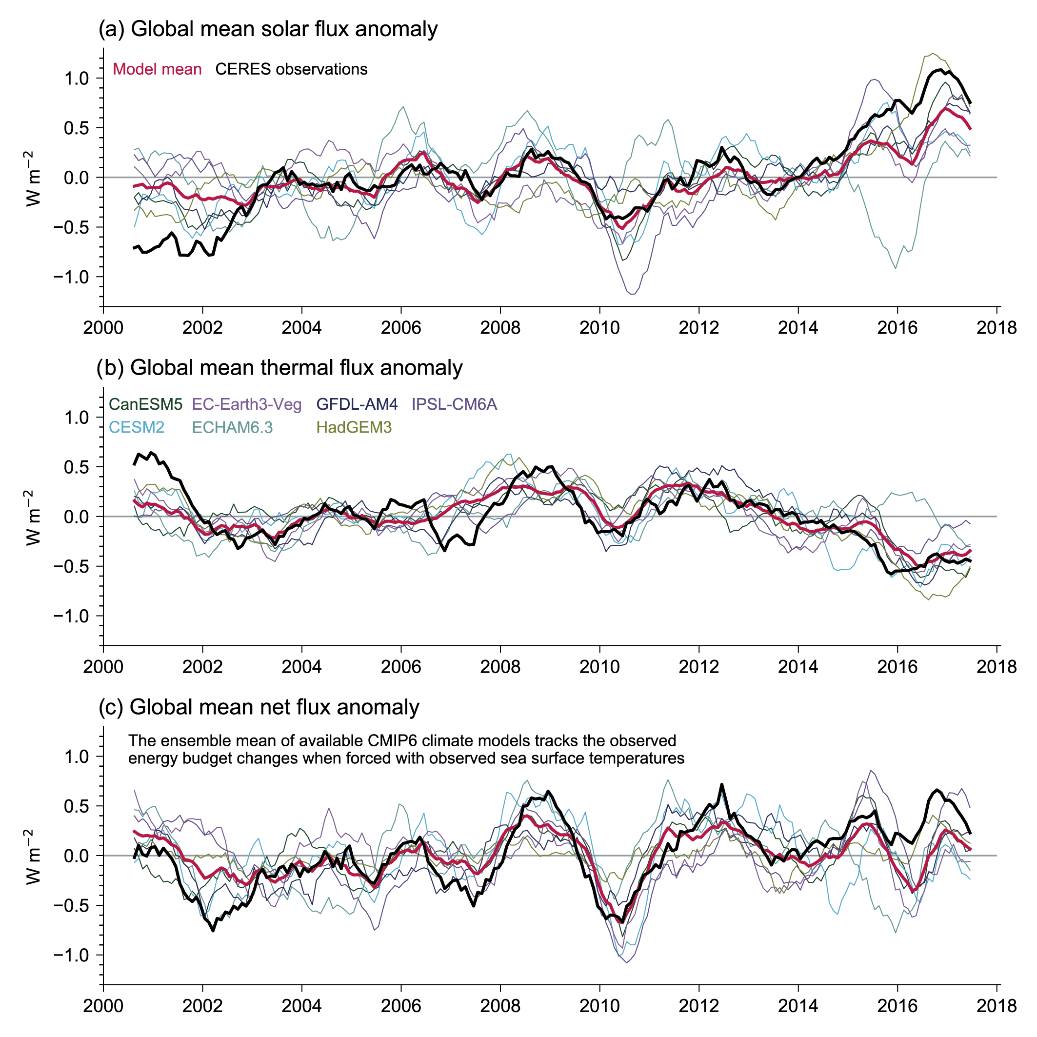
Satellite observations match the MODTRAN model very well, but they show the same radiative imbalance. See Fig. 4. The only explanation is that the “measurements” are actually calculated with algorithms similar to those in the model. The shapes of the green curve of the recursive model and the observations are identical, but the observations would have to be multiplied by the scale factor deduced from the recursive calculation to make everything fit.