DRAFT - The Climate Puzzle Pieced Together
There are two types of back-radiation. The first is thermal in nature. It has a significant influence on temperature. The second is fluorescence radiation, which has no effect.
1 Summary
In a previous paper, it was shown that back-radiation by greenhouse gases (GHGs) had no influence on the Earth’s surface temperature. This paper was later supplemented by an educational video posted on YouTube.
To my great disappointment, this article had very little impact. It was probably considered too simplistic. The atmosphere was not explicitly shown in the bathtub model. I considered a more complete model showing different energy reservoirs within the Earth-Atmosphere system (EAsys). See Section 2.
The IPCC claims that greenhouse gases create a radiation deficit that would cause an increase in temperature. This approach is flawed because it confuses internal and external energy flows. See Section 3.1 . It is based on a theory of radiative transfer that is incomplete and contains a less obvious, but very important, error. The Section 3.2 explains why the supposedly observed radiative deficit is only an illusion.
It remains to be explained why an Earth without an atmosphere would be about 33°C colder than the current Earth. I made a lot of assumptions and calculations to justify the current temperature, only to find myself in a dead end. The Earth had to absorb about twice as much energy as it receives. It seemed paradoxical.
I then re-evaluated the single-layer model, which I had always considered to be false. After careful consideration, I realized that my approach was flawed. There is more than a grain of truth in this model, which is correct. It is enough to introduce an additional parameter (the transparency of the atmosphere) for it to perfectly justify the current temperature. The interpretation of this model, however, is completely incorrect: the effect is based on Stefan-Bolzmann (SB) radiation, which has nothing to do with the fluorescence radiation characteristic of GHGs. See Section 3.3.
The back-radiation that we observe therefore has two natures. The first is thermal radiation that can only come from water in liquid or solid form present in the atmosphere, and the second is fluorescence radiation emitted by GHGs.
In the rest of this document, I will use the term TBR to refer to thermal back-radiation, and FBR to refer to fluorescence back-radiation. In the previously mentioned videos, the term back-radiation used only refers to FBR.
Similarly, we must differentiate between a thermal greenhouse effect (TGE) and a fluorescence greenhouse effect (FGE). The TGE is significant, and the FGE is zero.
Section 4 describes a complete model combining TGE and FGE, as well as evaporation/condensation and convection. Surprisingly enough, this model is Trenberth’s if we explicitly include the downward fluxes of latent heat and convection, abusively disguised and accumulated in an FBR.
Section 6 shows that our brain is not necessarily an objective guide when faced with complex analyses.
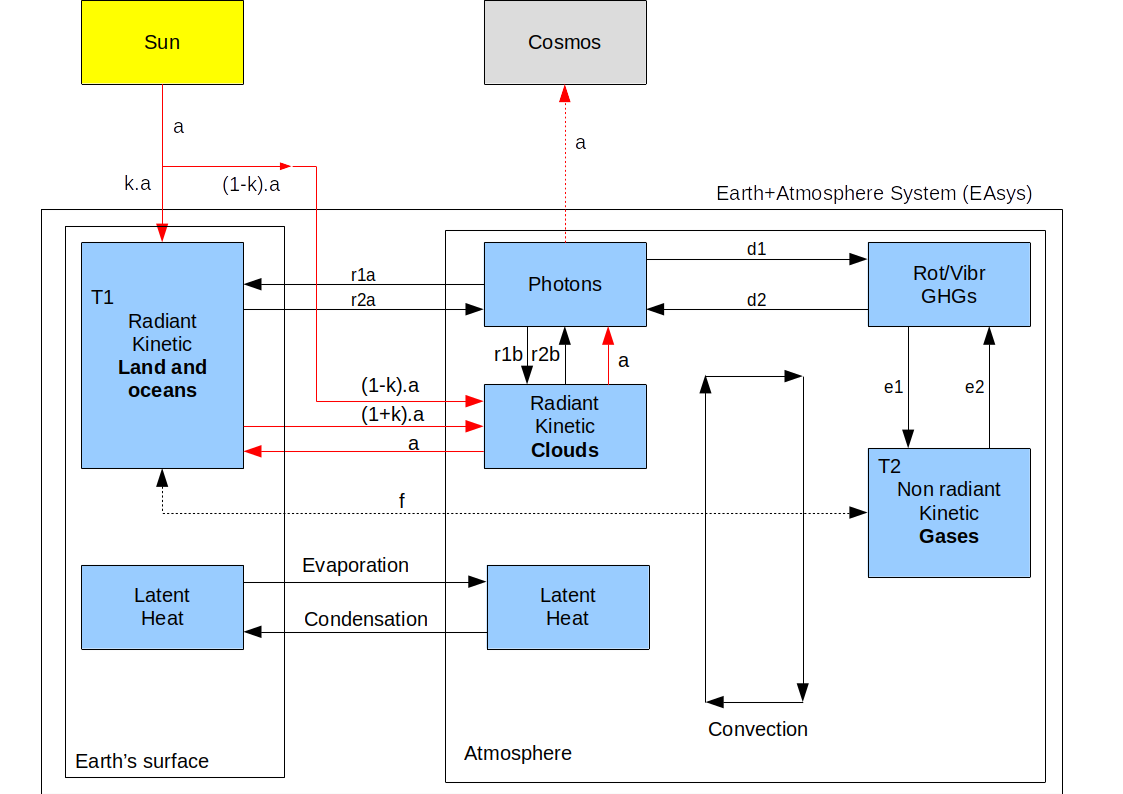
2 Modified diagram for a cloudless atmosphere
The Earth’s surface is considered to be a black body that emits thermal radiation according to the Stefan-Boltzmann (SB) law \(R = \sigma T_1^4\) . This radiation is considered to occur in a completely clear sky, without any clouds, and is not affected by the atmosphere, whether it contains GHGs or not. Evaporation/condensation is not taken into account. We are therefore within the framework of a purely radiative emission model, exactly as in Van Wijngaarden and Happer (2020). See Fig. 1.
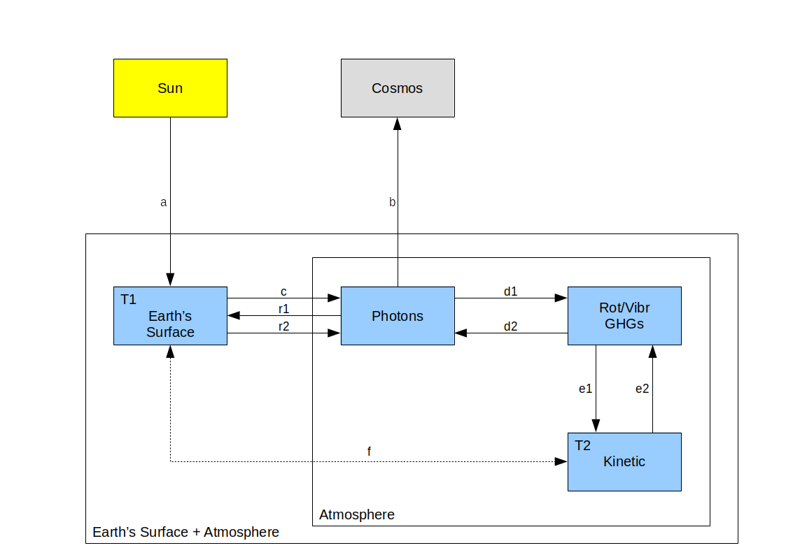
The rectangles represent reservoirs containing energy. The arrows represent energy flows between the reservoirs. The atmosphere is considered transparent to radiation from the Sun.
The yellow rectangle represents the Sun, part of whose radiation is absorbed by the Earth’s surface. The gray rectangle represents the Cosmos.
The rectangle Earth’s Surface represents the heat accumulated beneath the Earth’s surface. T1 is the temperature at this surface.
The rectangle Photons represents the energy of photons transiting through the atmosphere from the Earth’s surface and greenhouse gases.
The rectangle Rot/Vibr GHGs represents the variation in rotational/vibrational energy of greenhouse gas (GHGs) molecules relative to their unexcited ground state.
The rectangle Kinetic represents the translational kinetic energy (heat) of the molecules in the atmosphere. T2 is the temperature at the base of the atmosphere.
The flux a represents the portion of the solar flux absorbed by the surface of the Planet.
The flux b represents the flux emitted by the atmosphere towards the Cosmos.
The flux c corresponds to the thermal radiation emitted by the surface of the Planet. It depends only on the temperature T1.
Let’s review the mechanisms of action of GHGs. Their molecules can:
Increase their rotational/vibrational energy by absorbing a photon from the atmosphere ( flux d1 ).
Decrease their rotational/vibrational energy by emitting a photon into the atmosphere ( flux d2 ).
Increase their rotational/vibrational energy by borrowing translational kinetic energy from a neighboring molecule during an inelastic collision with it ( flux e2 ).
Decrease their rotational/vibrational energy by increasing the translational kinetic energy of a neighboring molecule during an inelastic collision with it ( flux e1 ).
The energy balance of each action mechanism is zero. The same is true for the atmosphere, as long as the photons involved do not leave it.
Photon emission by greenhouse gases can occur in any direction: it is isotropic. It is inevitable that some of these photons will be reflected back toward the Earth’s surface (flux r1).
The flux r2 represents a complementary flux emitted by the planet’s surface in response to the flux r1.
The flux f represents the heat exchanged by conduction between the planet’s surface and the atmosphere. It only exists when the temperatures T1 and T2 are different and flows in the direction from the hotter body to the colder one.
When the planet absorbs a constant portion of solar radiation, an equilibrium situation is eventually established.
The amount of energy contained in each of the reservoirs on the planet’s surface and in the atmosphere (the blue rectangles) stabilizes at a constant value. The temperatures T1 and T2 are equal, and the flux f is zero. For each of these reservoirs, the sum of the incoming fluxes is equal to the sum of the outgoing fluxes. If this were not the case, there would be a continual increase or decrease in the energy contained in certain reservoirs.
Let us assume, in the first phase, that the GHG molecules present in the atmosphere are all in their unexcited ground state and that the GHG action mechanisms are inhibited.
In this case, the fluxes r1, r2, d1, d2, e1, e2 are all zero.
The equilibrium of the Planet Surface reservoir implies that c = a.
The equilibrium of the Photon reservoir implies that b = c = a.
Under the action of absorbed solar radiation, heat accumulates under the Earth’s Surface, whose temperature increases until the flux c is equal to the flux a. At the same time, the Earth’s Surface heats the atmosphere by conduction, and energy accumulates in the Kinetic reservoir until the temperatures T1 and T2 equalize. The temperature T1 is determined by SB’s law, and the flux f is zero.
Let us now disinhibit the mechanisms of action of GHGs.
Let’s assume that temperatures T1 and T2 change to new values T’1 and T’2 and that T’1 = T’2 and f = 0. This is the situation we observe today with a current atmospheric CO2 concentration of over 400 ppm.
The equilibrium of the Earth’s Surface + Atmosphere reservoir implies that b = a. This is always true, whether there is a greenhouse effect or not.
The equilibrium of the Earth’s Surface reservoir implies that a + r1 = c + r2 = a + r2, since c = a.
It follows that r2 = r1: the surface re-emits the entire flux r1.
The equilibrium of the Photon reservoir implies c + r2 + d2 = b + r1 + d1, and therefore d2 = d1, since c = b = a and r2 = r1.
The equilibrium of the Rot/Vibr GHGs reservoir implies d1 + e2 = d2 + e1, and therefore e2 = e1, since d2 = d1.
The equilibrium of the Kinetic reservoir implies e1 = e2.
Therefore, all reservoirs contain the same energy, whether the GHGs are active or not. Therefore, the temperatures have not changed: T’1 = T1 and T’2 = T2.
Fig. 1 represents a system of communicating vessels connected 2 by 2. The flows a, b and c being equal, they cannot change the total internal energy of the system, nor can the GHGs which do not produce any energy and can only transfer energy between the reservoirs. These transfers have no impact on the individual contents of the reservoirs because they communicate with each other.
GHGs therefore do not influence the surface temperature T1, nor the temperature at the base of the atmosphere T2, nor the energy accumulated beneath the Earth’s surface and in the atmosphere. But can the temperature profile as a function of depth (oceans and land masses) or altitude (atmosphere) be affected?
For what happens beneath the surface, the answer is no. GHGs are absorbed in a surface layer of barely ten µm, whose temperature does not change. This is also the case for the atmosphere. This requires some additional considerations, as outlined in Section 3.2.
3 Some theories of the greenhouse effect
3.1 The IPCC approach
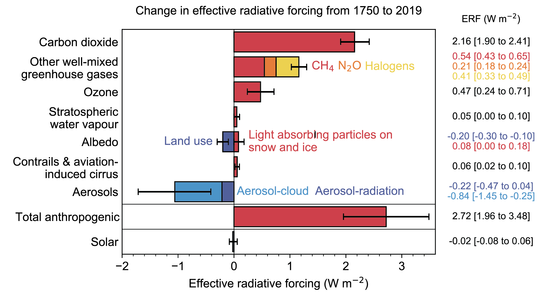
Based on radiative transfer analyses and simulation programs that are confirmed by satellite observations, the IPCC considers that the increase in GHGs since 1750 has caused a total radiative forcing of a few W/m2. See Fig. 2
The IPCC states that these radiative forcings have caused the Earth’s surface temperature to increase by about 1°C since 1750. See Fig. 3.
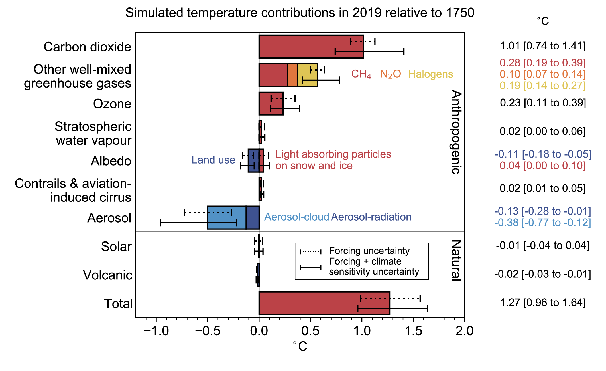
Almost all of the temperature increase observed since 1750 should therefore be attributed to radiative forcing caused by the increase in GHGs in the atmosphere, particularly that of CO2.
The IPCC established the figures for Fig. 2 and Fig. 3 based on studies and simulation programs.
Let’s take a moment to consider what happens when FBR photons return to the Earth’s surface.
GHG radiation is fluorescence radiation. Its nature is different from thermal SB radiation. These photons will only be absorbed by the surface if the surface exhibits absorption bands common to the GHG emission bands.
Water is ubiquitous on the Earth’s surface. It has absorption bands around 3 µm, 6 µm, and around 12 µm in a broad region that extends over a large portion of the radiation between 10 and 100 µm. Absorption in these bands will be followed by almost complete thermalization. In what follows, we will assume that the FBR is completely absorbed by the Earth’s surface, even if this is not the case. However, this has no impact on the surface temperature because the FBR flux is not external, but was previously emitted by the Earth’s surface. Fig. 4 helps to understand the difference.
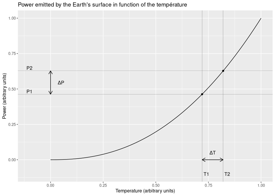
Those who believe that the FBR warms the Earth’s surface are making a serious conceptual error. They consider the point with coordinates T2, P2 to be the new equilibrium point because they assume that the FBR is cumulative with solar radiation. They confuse an internal incoming flux with an external flux, ignoring that the internal incoming flux is balanced by an internal outgoing flux of the same value. This invention of a complementary external flux is a flagrant violation of the principle of conservation of energy. A body at thermal equilibrium to which the same energy flux is added and removed will not change temperature if the external flux it absorbs remains constant.
If the RRF did indeed create an increase in temperature, we would have a runaway effect because each increase in temperature would cause an increase in the RRF, which in turn would induce a further increase in temperature, and so on. To prevent the temperature from diverging to infinity, there would have to be no further increase in the RRF beyond a certain temperature, contrary to what the online calculator MODTRAN from the University of Chicago shows.
The confusion between external and internal fluxes is not trivial, but what is even more serious is that the radiative forcing of GHGs is only an illusion. This is explained in the Section 3.2.
3.2 Theories based on radiative equilibrium (Schwarzschild equation)
In the lower atmospheric layers, the probability of a GHG molecule re-emitting a photon it has absorbed is very low, because the frequency of inelastic collisions is very high. At this location, if the flux e1 is greater than the flux e2 (see Fig. 1), there is an accumulation of kinetic energy, and an increase in temperature. The warmed and lighter air in the lower atmospheric layers will be carried to higher altitudes, which will bring cooler air back to lower altitudes. A convection circulation is established. At higher altitudes, the air is less dense and the probability of GHG re-emission increases. Thermalization of the lower atmospheric layers is a mechanism that allows energy to be transported higher into the atmosphere that would otherwise be trapped in the lower layers.
Quantifying these mechanisms is horribly complex. Some authors use the Schwarzschild equation to achieve this. This equation was described in Schwarzschild (1906) at the beginning of the previous century to calculate scattering and absorption in the solar atmosphere. In Van Wijngaarden and Happer (2020), the authors explain the calculation technique they use. The paper is very well written, and even though the calculations are complicated, the approach followed is clear.
The Earth’s surface is considered a black body with an average temperature of 15°C. Initially, the temperature at the base of the atmosphere is assumed to be equal to the surface temperature.
The calculations are based on a standard atmospheric temperature profile intended to represent today’s atmosphere with its current GHG concentrations and determine the impact of a doubling of CO2 on this standard profile.
The calculation is performed in two steps.
First, the Schwarzschild equation is used to calculate the distribution of radiative energy in the atmosphere under the effect of the GHG action mechanisms modeled in the HITRAN database. At the end of this phase, a radiation deficit is observed at the top of the atmosphere.
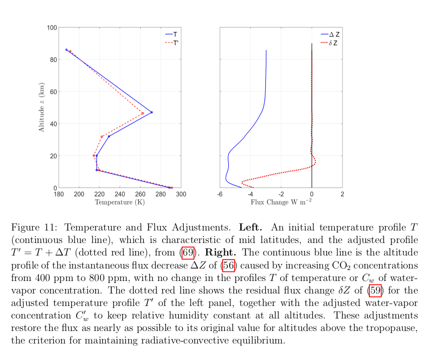
In a second phase, the temperature profile is adjusted to restore radiative balance. The temperature of the troposphere is increased while maintaining the initial adiabatic gradient, at the expense of a greater decrease in the temperatures of the higher atmospheric layers. See Fig. 5
Based on assumptions regarding the treatment of humidity in the calculations, the authors obtain a temperature increase at the base of the atmosphere of between 1.4 and 2.2°C for a doubling of CO2. They assume that there is a saturation effect and that additional doublings will have much less impact on atmospheric temperature.
The calculations do not go any further. No heat balance is taken into account for the Earth’s surface.
The problem is that we are now in a situation where the temperature at the base of the atmosphere is higher than the Earth’s surface temperature. However, no temperature difference is observed today, so it is not logical that there would be one after a doubling of CO2.
In the second phase of calculation corresponding to the readjustment of temperatures and fluxes, it would be necessary to take into account an additional constraint of equality of temperatures at the Earth’s surface and at the foot of the atmosphere. Since the RRF has no impact on the surface temperature, in the left figure, the red curve should start at the same point as the blue curve. Considering that the adiabatic gradient in the troposphere is not affected by GHGs, the first segment of the red curve should be identical to that of the blue curve, and the temperature adjustment could only be done on the 4 points located above the troposphere, ensuring that the energy balance is preserved. This leaves only a small margin of maneuver. There is every reason to believe that the rest of the red curve would be unchanged. In 1917 Einstein showed that the emission and absorption of radiation by molecules did not modify the distribution of their speeds. See Einstein (1917). It is therefore reasonable to assume that GHGs do not affect the local thermal balance anywhere, the principle of which is detailed in this article.
In any case, an observer placed in the troposphere will not feel any temperature difference after a doubling of CO2.
If we do not make these adjustments, we can estimate how a warmer atmosphere will warm the Earth’s surface. Since the heat capacity of the oceans is significantly greater than that of the atmosphere, after exchanging its excess heat, the temperature of the atmosphere will be equal to that of the ocean, which will hardly change. The final equilibrium temperature of a closed system where the entire atmosphere is at 21 °C and in contact with an oceanic layer of barely 50 m at 20 °C, is equal to 20.05 °C (Remember that the average depth of the oceans is about 3800 m). See the calculation note atmosphere-ocean. This final warming is imperceptible.
There is another strong inconsistency in the Van Wijngaarden and Happer (2020) model. It is also found in the MODTRAN calculator. It concerns the high-altitude emission spectra. See Fig. 6.
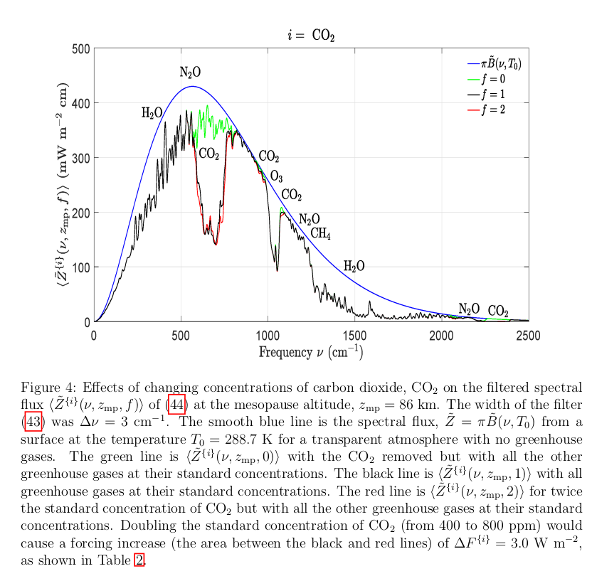
The blue curve in this figure represents the SB radiation emitted by the surface at a temperature of 288.7°K. For a transparent atmosphere, without GHGs, the same curve would be found at the top of the atmosphere, estimated at an altitude of 86 km.
The black curve represents the theoretical radiation resulting from the Schwarzschild equilibrium for current GHG concentrations. This can only correspond to the first calculation phase mentioned above, before the fluxes were restored. After this, the surfaces below the blue and black curves should be identical. The black curve should exhibit peaks and troughs relative to the blue curve. The Earth and the atmosphere have had sufficient time to adapt to current GHGs concentrations.
These considerations also apply to the green and red curves.
In Van Wijngaarden and Happer (2020), in section 8, the authors compare the modeled radiation intensities with satellite observations. See Fig. 7.
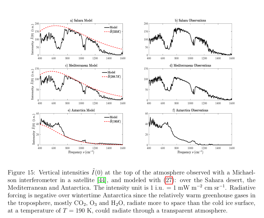
The correspondence is excellent, but here too it is unclear why the areas under the red and black curves in the left panel are not equal. The only explanation is that the “observations” in the right panel are based on the same faulty algorithms as those used in the left panel.
The re-emission of the FBR is done at a constant temperature throughout the entire wavelength range. It can be done several times. This allows to bypass the more absorbing bands by passing through less absorbing bands. This is explained in this short but very important document. This iterative processing should be used in the first calculation phase of Van Wijngaarden and Happer (2020). The second phase is then superfluous since the fluxes are already correct and there is therefore no temperature adjustment to be made.
3.3 The one-layer model
In this model, the greenhouse effect is explained by the interaction of two plates that behave like black bodies. The first plate represents the Earth’s surface, the upper surface of which is perfectly absorbent, and the lower surface of which is perfectly thermally insulated. This model is taught in various universities and disseminated by academic institutions. It is the basics of the greenhouse effect. See for example (Dufresne and Treiner 2011).
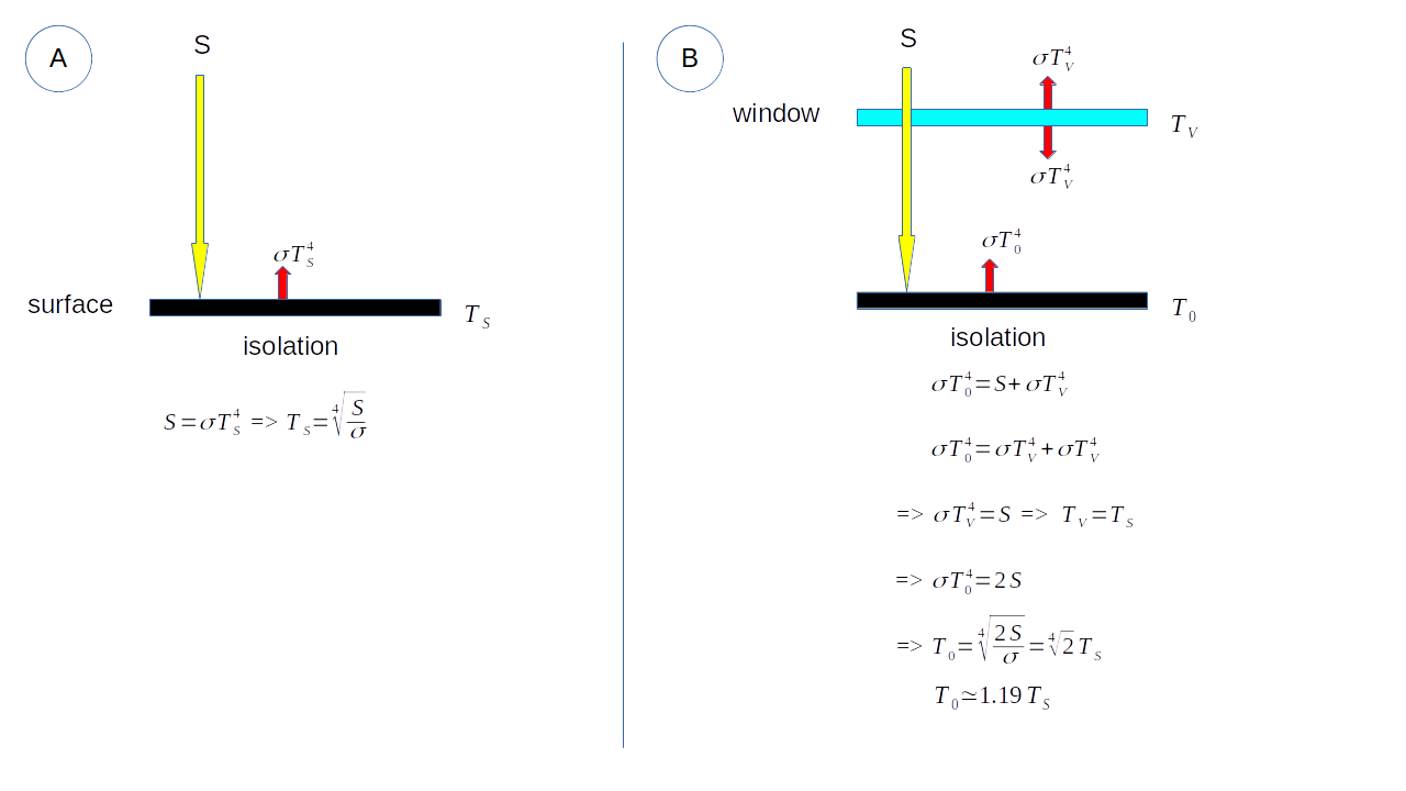
The second plate represents the atmosphere. It is placed above the first. It is a pane of glass that is completely transparent to solar radiation and completely absorbs the infrared radiation emitted by the Earth’s surface and re-emits it upwards and downwards. The pane is considered isothermal.
By calculating the thermal balance of each plate, we observe that:
the temperature of the pane is equal to the surface temperature in the absence of an atmosphere.
the surface receives radiation equal to twice that in the absence of an atmosphere, with the downward radiation from the pane adding to that of the sun. By applying SB’s formula, the surface temperature is approximately 1.19 times the temperature of the pane.
Taking albedo into account, the authors obtain a surface temperature of -15°C without an atmosphere and +30°C with an atmosphere, while the current average temperature is closer to 19°C.
This model is based on pure thermal radiation (SB) exchange. In the atmosphere, only liquid or solid water present in clouds can emit this type of thermal radiation. This model describes an “atmosphere effect” that has nothing to do with the fluorescence radiation characteristic of GHGs. I adapted it to correct the overestimation of surface temperature (see here), but this does not change the principle. There are no GHGs in this model. It is therefore difficult to see where more could be added.
4 Complete diagram
It is obtained by combining the FGE and the TGE, and adding latent heat fluxes (water cycle) and a convection loop. See Fig. 9.
Heat fluxes
Part of the incident solar radiation is reflected by the atmosphere and its clouds, and by the Earth’s surface. The EAsys absorbs a flux a from the Sun. A flux of the same value (red dotted line) is emitted towards the Cosmos after passing through the atmosphere. The spectral composition of this flux has been modified by GHGs, without changing its overall intensity. See the green curve in this figure.
A fraction k.a is absorbed by land and oceans, and a fraction (1-k).a is absorbed by clouds in the atmosphere.
Clouds emit a flux a into space, and another flux a absorbed by the Earth’s surface. The Earth’s surface emits a flux (1+k).a which is absorbed by the clouds.
Fluxes associated with GHGs
The fluxes r1 and r2 in Fig. 1 have been renamed r1a and r2a. Analogous fluxes r1b and r2b have been introduced to describe the interaction of GHGs with clouds. As before, the sums of the fluxes r1a and r2a, r1b and r2b, d1 and d2, e1 and e2, are zero.
Other fluxes
The conduction flux f is zero.
Convection is an internal loop that does not affect the overall balance.
The latent heat fluxes offset each other: on average, there is as much evaporation as condensation returning to the surface through rain.
Conclusions of this diagram
Only the red fluxes corresponding to the TGE play a role in the energy balance of the EAsys which is explained by the extended 1-layer model described here.
This energy balance is that of Figure 1 in Trenberth, Fasullo, and Kiehl (2009) as long as it is interpreted correctly. See Fig. 10.
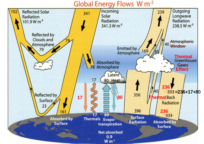
Let us take the values displayed in Trenberth’s energy balance.
The Surface Radiation of 396 W/m2 is that of a black body at a temperature of 16 °C, of which a portion of 40 W/m2 escapes directly into space through the Atmospheric Window.
A radiation of 239 W/m2 is absorbed by the EAsys (161 W/m2 Absorbed by Surface and 78 W/m2 Absorbed by Atmosphere. These figures were retained by Trenberth on the basis of numerous analyses.).
The diagram only shows the ascending fluxes of latent heat (Evapo-transpiration = 80 W/m2) and convection (Thermals = 17 W/m2).
An Outgoing Longwave Radiation of 239 W/m2 is measured at the top of the atmosphere.
There is a Net Absorbed value of 1 W/m2, justifying the current observed warming.
The Back Radiation of 333 W/m2 is calculated to balance the balance: 333=356+80+17+78-169-30+1. This term therefore includes the downward convection fluxes (17 W/m2) and latent heat fluxes (80 W/m2) which are assimilated to the action of GHGs!!!. These downward fluxes must be considered separately (orange and blue arrows added to the original diagram), and the Back Radiation then increases to 236 W/m2 (333-17-80).
By blocking the atmospheric window which is very symbolic (See here), the atmosphere emits 239 W/m2 upwards and almost the same thing downwards (236 W/m2), as in the one-layer extended model.
The parameter k of this model can be calculated in 2 ways which produce almost the same result:
Either by calculating the ratio between the radiation absorbed by the surface (161 W/m2) and the total radiation absorbed (239 W/m2), which gives a value of 0.67.
Or by decreasing by one unit the ratio between the radiation emitted by the surface (396 W/m2) and the total radiation absorbed (239 W/m2), which gives a value of 0.66.
The Trenberth diagram can therefore be perfectly interpreted as a thermal greenhouse effect justified by a very simple model which explains the temperatures observed by the thermal radiation of liquid and solid water present in the atmosphere, without any influence of GHGs.
5 Experimental simulations
5.1 Experimental Setup
The experiments are conducted using a setup consisting of two communicating reservoirs. The second reservoir is equipped with a drain port. See Fig. 11.
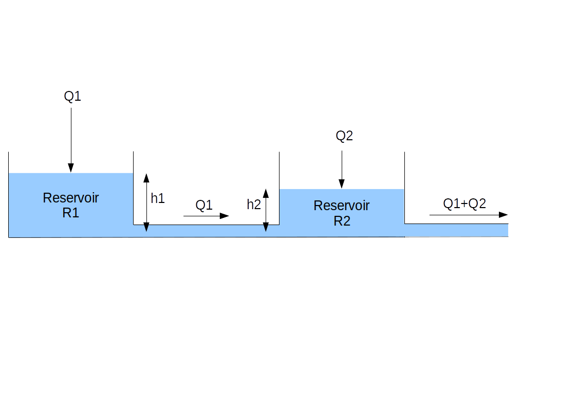
Given:
Q1 the supply flow rate of tank R1
Q2 the supply flow rate of tank R2
Q = Q1 + Q2 the total supply flow rate
k = Q1/Q the fraction of the total flow feeding the reservoir R1.
h1 the water height in tank R1
h2 the water height in tank R2
s1 the cross-sectional area of the pipe connecting the two tanks
s2 the cross-sectional area of the tank drain R2
g the acceleration due to gravity
k is the equivalent of the degree of transparency of the atmosphere in the extended 1-layer model.
The heights h1 and h2 can be calculated by Torricelli’s Formula.
\[ h2=(Q1+Q2)^2/(2~ g~ s2^2) \tag{1}\]
The water height h2 depends only on the total flow rate and s2.
\[ \begin{align} h1-h2&=Q1^2/(2~g~s1^2) \\ & = k^2 Q^2/(2~g~s1^2) \end{align} \tag{2}\]
The height difference depends only on Q1 and s1. It is the equivalent of the TGE in the 1-layer model. It is zero if Q1=0. It is almost zero if the section s1 is very large.
It is maximal when k=1, as in the extended one-layer model.
5.2 FGE in a cloudless atmosphere (no TGE)
The basic experimental setup is done with a large surface area s1. This cancels the TGE. In the Fig. 9, the Clouds reservoir disappears. Omitting the latent heat and convection fluxes which have no effect, this brings us back to Fig. 1. Since the 3 atmospheric reservoirs are constant, they can be replaced by a single reservoir. A pump rejecting the water it sucks from reservoir R2 into reservoir R1 will simulate the FGE. See Fig. 12.
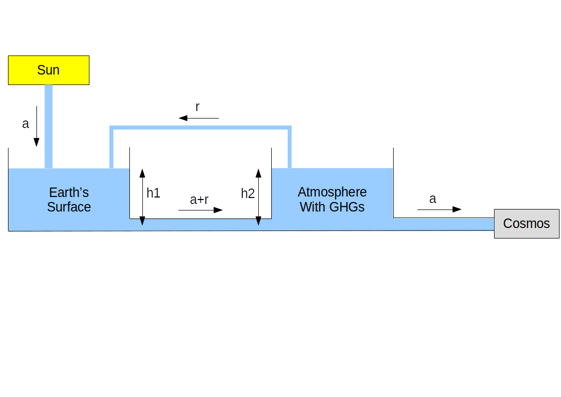
The first reservoir represents the energy stored by the Earth’s surface, and the second the energy stored in the atmosphere. The first reservoir is supplied by a tap whose flow rate symbolizes the solar energy absorbed by the Earth’s surface (flow a). The pipe connecting them allows for a bidirectional radiative exchange between them.
The second reservoir is equipped with a drain port. The water escaping from it represents the energy emitted into space. A pump draws water from the second reservoir and reinjects it into the first. Its flow rate symbolizes the back-radiation (flow r).
A flow rate a + r passes through the pipe connecting the two reservoirs.
The water heights h1 and h2 symbolize the temperatures of each reservoir.
This diagram is equivalent to that of Panel C in the initial version of the GHG analysis. Simply replace a with 1, r with f and split the flow a + r = 1 + f into a flow 1 and a flow f.
The back-radiation photons may have been created within the atmosphere, and will generally not be the same as those emitted by the surface of the Planet. This fully addresses the objection made by William Happer (see Note 1), and the comparison with rain remains valid. It is sufficient to reason in terms of energy extracted and reinjected in the context of two communicating reservoirs.
I asked William Happer, an internationally renowned scientist, what he thought of the first video, reminding him of the comparison with rain, which has no influence on ocean levels since it comes from evaporation from their surface.
Here’s what he told me:
I too don’t think back-radiation at the Earth’s surface is particularly useful for understanding greenhouse warming. But there is no doubt that back-radiation exists. You can measure it with a hand-held radiometer.
I don’t think there is anything wrong with your metaphor of water filling leaking reservoirs, but you have to keep in mind that photons are not like water molecules that are not created or destroyed in the cycle of evaporation and precipitation. Photons are routinely created and destroyed. You don’t need to have a “zero sum game” for photons.
The back-radiation at Earth’s surface is not from backscattered photons that were previously emitted from the surface. Rather, the back-radiation consist of photons that were created at the expense of the thermal energy of the atmosphere by greenhouse molecules or clouds. Much of the thermal energy came from upward convection of warm air, not from surface thermal radiation.
Several experiments based on a setup consistent with this simplified scheme have been filmed. They fully confirm that the FBR does not affect the thermodynamic equilibrium of the planet’s surface and atmosphere. The corresponding video has been published on YouTube.
5.3 The TGE in an atmosphere with clouds
The basic experimental setup is designed with a small surface area s1 to ensure a clearly defined TGE. This setup corresponds to panel B of this figure.
A cuvette collecting the feed flow is placed at the top of the basic setup. Its bottom contains holes that distribute the flow between the reservoirs, thus simulating the transparency degree k of the atmosphere.
This setup shows that the surface temperature is maximum when k=1, and that it decreases with the value of k.
It is not possible to simulate the FGE as in Fig. 12, unless working with two synchronized pumps (one from R1 to R2, and the other from R2 to R1). In this trivial case, it is obvious that the FGE has no influence on the levels.
If we work with a single pump that draws and delivers a flow rate of r, we are not simulating an FGE, but we are changing the transparency degree k of the TGE. If we start from a situation with flow rates Q1 and Q2, activating flow rate r will simulate a situation with Q’1=Q1+r and Q’2=Q2-r. The k parameter increases, and if r > Q2, we could even simulate the completely unrealistic case of a transparency degree k greater than 1.
A video corresponding to this setup has also been published on YouTube.
6 Our brain sometimes plays tricks on us
The same experimental setup can demonstrate the FGE and the TGE by simply adjusting the cross-section of the connecting duct between the two compartments. This now seems obvious, but my mind played a few tricks on me before I reached this conclusion.
When I began writing this article, my goal was to demonstrate the non-existence of the FGE using the setup shown in Fig. 12.
Unknowingly, I had actually created the Fig. 11 setup with Q2=0 and a small s1 section. I was very disconcerted when I observed a difference in level between the two compartments. It was a big surprise. I expected to observe a zero level difference, which would have been consistent with the first video mentioned at the beginning of this document.
When I activated the pump to simulate the greenhouse effect, the level difference increased without affecting the water level in the right compartment representing the atmosphere. I thought this setup didn’t reflect reality since I was observing a temperature discontinuity between the Earth’s surface and the one at the base of the atmosphere, which doesn’t exist in reality.
I had just observed the TGE without knowing it.
I created a new setup with a much larger s1 cross-section, and everything was back to normal. I mistakenly attributed my initial observations to pressure drops in the system.
Like others before me, I had convinced myself that the plates in the single-layer model must have the same temperature. I even started writing an article on this subject.
I couldn’t understand the Trenberth diagram, and I tried to justify the observed temperatures without resorting to a greenhouse effect. Without success. It was only then that I carefully re-evaluated the single-layer model, only to realize that I had made a mistake in my reasoning. It was easy to add an atmospheric transparency parameter to adjust this model to the observed temperatures.
It was only then that I set up the equations for the experimental setup, and everything became clear to me.
There are therefore two types of greenhouse effects: an FGE and an TGE.
The FGE has no influence on temperatures. The measured FBR comes only from fluorescence photons emitted in the immediate vicinity of the measuring device.
The TGE is caused by thermal radiation from liquid or solid water contained in clouds. It propagates throughout the atmosphere and has a strong impact on temperatures. It is not dependent on GHGs.
The principles of the one-layer model and the Trenberth diagram are correct, but their interpretation is incorrect: GHGs are not involved at all.
I firmly believe that the climate puzzle has been pieced together: the proposed model is consistent with observations.
7 Conclusions
The conclusions of my previous article are still relevant. See here.
In the meantime, the situation has worsened.
Virtuous Europe, champion of democracy, has been caught red-handed, funding external organizations to spread climate alarmism.
The International Court of Justice (ICJ) has issued an advisory opinion affirming that states have a legal obligation to protect the climate and reduce greenhouse gas emissions.
In 1859, John Tyndall concluded that gases in the atmosphere influence the climate.
In 1896, Svante August Arrhenius estimated that a doubling of CO2 would cause a temperature increase of 5°C.
Since 1972, IR radiation spectra measured by satellite at the top of the atmosphere have reportedly shown a huge, inexplicable radiation deficit.
Since then, climatology has developed based on these scientific errors, which can be explained by
A confusion between an internal flow and an external flow.
Another confusion between thermal radiation and fluorescence radiation. The back-radiation we measure is a mix of thermal radiation and fluorescence radiation. The first type of back-radiation can have an impact on temperatures. This thermal back-radiation can only come from non-gaseous water present in the atmosphere, regardless of atmospheric GHG concentrations. Fluorescence back-radiation due to GHGs has no influence on the temperature of the Earth’s surface.
A radiative transfer theory that we forget to apply recursively. When it is applied only once, it leads us to believe in the existence of an illusory radiative deficit, confused with an external flux that would warm the Planet. When it is applied recursively, we see that this radiative deficit does not exist.
In this issue, I experienced a first HaHa moment when I realized that back-radiation due to GHGs originates at the Earth’s surface and doesn’t fall from the sky, coming from nowhere. I then rushed to write the article mentioned at the beginning of this one. It didn’t have the success I had hoped for.
After a phase of intense discouragement, I decided to write a more detailed version. All that remained was to find the flaw in the Schwarzschild equation used in particular in Van Wijngaarden and Happer (2020). As I reread this article for the umpteenth time, I experienced a second HaHa moment when I discovered that the model and observation graphs exhibited a significant energy imbalance that could easily be corrected by recursively applying this radiative transfer theory. Suddenly, the radiative forcings had disappeared.
But what is a HaHa effect? It is described by mathematician Martin Gardner in his book “Haha, ou l’éclair de la compréhension mathématique.” It occurs when a seemingly complicated problem has a very simple logical solution.
For example, it is impossible to place dominoes on a chessboard that cover exactly two adjacent squares while leaving two of the same color free. This could be verified by testing all the possible combinations, the number of which is enormous. It is much easier to consider that since each domino covers exactly one black and one white square, the remaining squares must necessarily be of opposite colors. Haha.
Faced with an even more complicated problem, the IPCC claims to have found a solution. It is apparently contained in a 2,400-page document containing 14,000 references and 39 computer models, which allegedly show that the Earth is warming under the action of fluorescence radiation. As paradoxical as it may seem, fluorescence back-radiation has no impact on the Earth’s surface temperature and creates no radiation deficit at the top of the atmosphere. The climate control knob (CO2) is broken. It is irreparable.
I hope I’ve managed to explain my HaHa moments and that everything is now much clearer. This article should trigger a tsunami of scientific truth against which fact-checkers will be powerless.
Of course, I don’t benefit from any scientific aura: I’m no match. Everything would be simpler if a renowned scientist shared my views. I resumed the discussion with W. Happer. During the first exchanges, he responded immediately with vague and highly unconvincing arguments. Then I had this second HaHa effect. I told him that his graphs showed a huge radiative imbalance. I haven’t heard from him in a few weeks. For now, I have few illusions. It’s a shame; I appreciated W. Happer’s courageous positions, but he could do much better in light of my arguments.
During my discussion with W. Happer, he explained that his main goal was to propose an explanation of radiative transfer and that his temperature increases for a doubling of CO2 had been overestimated to satisfy the requirements of peer review. He is a “lukewarm warmist” who believes that the temperature will increase by less than 1°C if CO2 is doubled. Hopefully, this last sentence will be changed to the imperfect tense soon.
Generally, climate realists are content to downplay the impact of greenhouse gases on the climate. Now, they can go on the offensive. Clintel should seriously consider this possibility, now that the IPCC’s position is patently false.
If nothing changes, I will end up believing that 97% of scientists actually believe in anthropogenic climate change, and that climatology, embroiled in a phase of Lysenkoism to the tenth power, will remain in its current state of total disrepair. Only 3% of clear-sighted minds profoundly disagree with the IPCC ?

As far as I’m concerned, the verdict is clear.

The latest images were generated by artificial intelligence (AI). It only took a few sentences to describe them. It’s truly impressive.
I had a long conversation with Gemini, Google’s AI, about climate change. I felt like I was conversing in natural language with a scholar with incredibly extensive knowledge. But when confronted with its own contradictions, the AI constantly regurgitates variations of its arguments. It has no self-learning capacity. Fortunately, otherwise the ultimate stage of evolution would be reached, and we would have to rely only on the benevolence of AI to preserve a far too cumbersome humanity that consumes so much of the energy it so desperately needs.
Retraining AIs is essential. They are becoming the new oracles, the sole custodians of THE Truth, and no debate, scientific or otherwise, will be possible. It’s terrifying.
PS
A list of arguments against the action of GHGs on the climate can be found here.
A list of arguments that show the impact of the Sun on the climate can be found here.
The model of a leaky container being fed with water may seem very naive. In reality, it is very relevant. The differential equation of this model is analogous to that of a simple thermal model of the climate at every point on the planet. This is explained here.